
Introduction
This notebook is for the workshop (Open Source Geospatial Workflows in the Cloud) presented at the AGU Fall Meeting 2025.
GeoAI represents the intersection of geospatial science and artificial intelligence, combining the power of machine learning with geographic information systems (GIS) to analyze, understand, and predict spatial patterns. This rapidly growing field enables us to extract meaningful insights from satellite imagery, aerial photos, and other geospatial datasets at unprecedented scales and accuracy levels.
The GeoAI Python package (https://
Data Preprocessing: Automated handling of various geospatial data formats, coordinate systems, and multi-spectral imagery
Model Training: Pre-configured deep learning architectures optimized for geospatial tasks like semantic segmentation and object detection
Feature Extraction: Automated extraction of geographic features from satellite and aerial imagery
Visualization: Interactive mapping and analysis tools for exploring results
In this workshop, you will:
Discover the core capabilities of the GeoAI package, including data preprocessing, feature extraction, and geospatial deep learning workflows
See live demonstrations on applying state-of-the-art AI models to satellite and aerial imagery
Learn how to train custom segmentation models for surface water mapping using different data sources
Explore real-world use cases in building footprint extraction and surface water mapping
Additional Resources
Deep Learning Architectures and Encoders
Before moving into the hands-on work, it’s important to first understand the key ideas behind deep learning architectures and encoders.
A deep learning architecture is like the blueprint of a factory. It defines how the network is organized, how data flows through different components, and how raw inputs are transformed into meaningful outputs. Just as a factory blueprint specifies where materials enter, how they are processed, and where finished products come out, a neural network architecture lays out the arrangement of layers (neurons) that progressively extract and refine patterns from data—for example, detecting cats in images or translating between languages.
Within this blueprint, an encoder functions as a specialized assembly line. Its role is to take messy raw materials (input data) and refine them into a compact, standardized representation that is easier for the rest of the system to work with. Some architectures also include a decoder assembly line, which reconstructs or generates the final output from the encoder’s compressed representation—for example, assembling a finished car from engine parts and panels.
In short:
Model architecture = the factory blueprint (overall design and flow)
Encoder = the preprocessing line (condenses raw inputs into useful parts)
Decoder = the finishing line (turns encoded parts into a final product)
Types of Architectures
Different blueprints are suited for different tasks:
Feedforward Neural Networks: simple, one-directional flow of data.
Convolutional Neural Networks (CNNs): specialized for images, capturing spatial patterns like edges and textures.
Recurrent Neural Networks (RNNs): designed for sequences, such as speech or time series.
Transformers: powerful models for language and beyond, using attention mechanisms (e.g., ChatGPT).
What Does an Encoder Do?
An encoder is the part of a neural network that takes an input (like an image or a sentence) and compresses it into a smaller, meaningful form called a feature representation or embedding. This process keeps the essential information while filtering out noise.
For example, the sentence “I love pizza” might be converted by an encoder into a vector of numbers that still reflects its meaning, but in a way that is easier for a computer to analyze and use.
Encoders appear in many contexts:
Autoencoders: learn to compress and reconstruct data.
Transformer Encoders: such as BERT, used for language understanding.
Encoder–Decoder Models: such as translation systems, where the encoder reads one language and the decoder generates another.
Encoders and Architectures in Practice
The pytorch segmentation models library provides a wide range of pre-trained models for semantic segmentation. It separates architectures (the blueprint) from encoders (the feature extractors):
Architectures:
unet,unetplusplus,deeplabv3,deeplabv3plus,fpn,pspnet,linknet,manet.Encoders:
resnet34,resnet50,efficientnet-b0,mobilenet_v2, and many more.
The GeoAI package builds on this library, offering a convenient wrapper so you can easily train your own segmentation models with a variety of architectures and encoders.
Environment Setup
You can run this notebook locally or in Google Colab. You will need a GPU for training deep learning models. If you don’t have a GPU, you can use the free GPU in Google Colab.
To install the GeoAI package, it is recommended to use a virtual environment. Please refer to the GeoAI installation guide for more details.
Here is a quick start guide to install the GeoAI package:
conda create -n geo -c conda-forge mamba
conda activate geo
mamba install -c conda-forge python=3.12 geoai
If you have a GPU, you can install the package with GPU support:
mamba install -c conda-forge geoai "pytorch=*=cuda*"You can install the package using pip:
pip install geoai-pyUse Colab GPU
To use GPU, please click the “Runtime” menu and select “Change runtime type”. Then select “T4 GPU” from the dropdown menu. GPU acceleration is highly recommended for training deep learning models, as it can reduce training time from hours to minutes.
Install packages
Uncomment the following cell to install the package. It may take a few minutes to install the package and its dependencies. Please be patient.
# %pip install geoai-pyImport libraries
Let’s import the GeoAI package.
import geoaiSurface water mapping with non-georeferenced satellite imagery
Surface water mapping is one of the most important applications of GeoAI, as water resources are critical for ecosystem health, agriculture, urban planning, and climate monitoring. In this first demonstration, we’ll work with non-georeferenced satellite imagery in standard image formats (JPG/PNG), which is often how satellite imagery is initially distributed or stored.
Why start with non-georeferenced imagery?
Many datasets and online sources provide satellite imagery without embedded geographic coordinates
It demonstrates the core computer vision aspects of GeoAI before adding geospatial complexity
The techniques learned here can be applied to any imagery, regardless of coordinate system
It’s often faster to iterate and experiment with standard image formats
We’ll use semantic segmentation, a deep learning technique that classifies every pixel in an image. Unlike object detection (which draws bounding boxes), semantic segmentation provides precise pixel-level predictions, making it ideal for mapping natural features like water bodies that have irregular shapes.
Download sample data
We’ll use the waterbody dataset from Kaggle, which contains 2,841 satellite image pairs with corresponding water masks. This dataset is particularly valuable because:
Diverse geographic coverage: Images from different continents and climate zones
Varied water body types: Lakes, rivers, ponds, and coastal areas
Multiple seasons and conditions: Different lighting conditions and seasonal variations
High-quality annotations: Manually verified water body masks for training
Credits to the author Francisco Escobar for providing this dataset.
I downloaded the dataset from Kaggle and uploaded it to Hugging Face for easy access:
url = "https://huggingface.co/datasets/giswqs/geospatial/resolve/main/waterbody-dataset.zip"out_folder = geoai.download_file(url)
print(f"Downloaded dataset to {out_folder}")The unzipped dataset contains two folders: images and masks. Each folder contains 2,841 images in JPG format. The images folder contains the original satellite imagery, and the masks folder contains the corresponding surface water masks in binary format (white pixels = water, black pixels = background).
Dataset characteristics:
Total image pairs: 2,841 training examples
Image format: RGB satellite imagery (3 channels)
Mask format: Binary masks where 255 = water, 0 = background
Variable image sizes: Ranging from small 256x256 patches to larger 1024x1024+ images
Global coverage: Samples from diverse geographic regions and water body types
Train semantic segmentation model
Now we’ll train a semantic segmentation model using U-Net architecture with a ResNet34 encoder and ImageNet pre-trained weights. Let’s break down these important choices:
Architecture: U-Net
U-Net is a convolutional neural network architecture specifically designed for semantic segmentation
It has a “U” shape with an encoder (downsampling) path and a decoder (upsampling) path
Skip connections between encoder and decoder preserve fine-grained spatial details
Originally designed for medical image segmentation, it works exceptionally well for geospatial applications
Encoder: ResNet34
ResNet34 is a 34-layer Residual Network that serves as the feature extraction backbone
Residual connections allow training of very deep networks without vanishing gradient problems
Balances model complexity with computational efficiency (deeper than ResNet18, more efficient than ResNet50)
Well-suited for satellite imagery feature extraction
Pre-trained weights: ImageNet
Transfer learning from ImageNet provides a strong starting point for feature extraction
ImageNet-trained models have learned to recognize edges, textures, and patterns relevant to natural imagery
Significantly reduces training time and improves performance, especially with limited training data
The encoder starts with knowledge of general image features, then specializes for water detection
Key training parameters:
num_channels=3: RGB satellite imagery (red, green, blue bands)num_classes=2: Binary classification (background vs. water)batch_size=32: Process 32 images simultaneously for efficient GPU utilizationnum_epochs=3: Training iterations (limited for demo; real-world would use 20-50+ epochs)learning_rate=0.001: Controls optimization step sizeval_split=0.2: Reserve 20% of data for validation to monitor overfittingtarget_size=(512, 512): Standardize all images to 512x512 pixels for consistent processing
For more details on available architectures and encoders, please refer to https://
# Test train_segmentation_model with automatic size detection
geoai.train_segmentation_model(
    images_dir=f"{out_folder}/images",
    labels_dir=f"{out_folder}/masks",
    output_dir=f"{out_folder}/unet_models",
    architecture="unet",  # The architecture to use for the model
    encoder_name="resnet34",  # The encoder to use for the model
    encoder_weights="imagenet",  # The weights to use for the encoder
    num_channels=3,  # number of channels in the input image
    num_classes=2,  # background and water
    batch_size=16,  # The number of images to process in each batch
    num_epochs=3,  # training for 3 epochs to save time, in practice you should train for more epochs
    learning_rate=0.001,  # learning rate for the optimizer
    val_split=0.2,  # 20% of the data for validation
    target_size=(512, 512),  # target size of the input image
    verbose=True,  # print progress
)
In the model output folder unet_models, you will find the following files:
best_model.pth: The best model checkpoint (highest validation IoU)final_model.pth: The last model checkpoint from the final epochtraining_history.pth: Complete training metrics for analysis and plottingtraining_summary.txt: Human-readable summary of training configuration and results
Evaluate the model
Model evaluation is crucial for understanding how well our trained model performs. We’ll examine both the training curves and quantitative metrics to assess model quality and identify potential issues like overfitting or underfitting.
Key evaluation metrics for semantic segmentation:
Loss: Measures how far the model’s predictions are from the ground truth
Training loss: How well the model fits the training data
Validation loss: How well the model generalizes to unseen data
Ideal pattern: Both should decrease, with validation loss closely following training loss
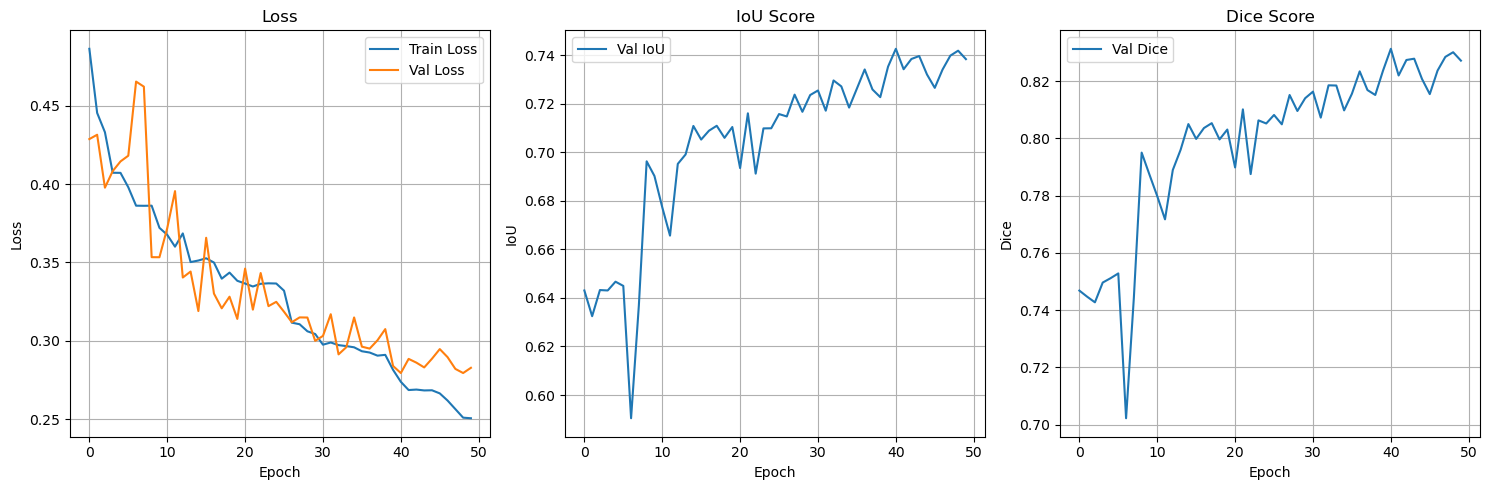
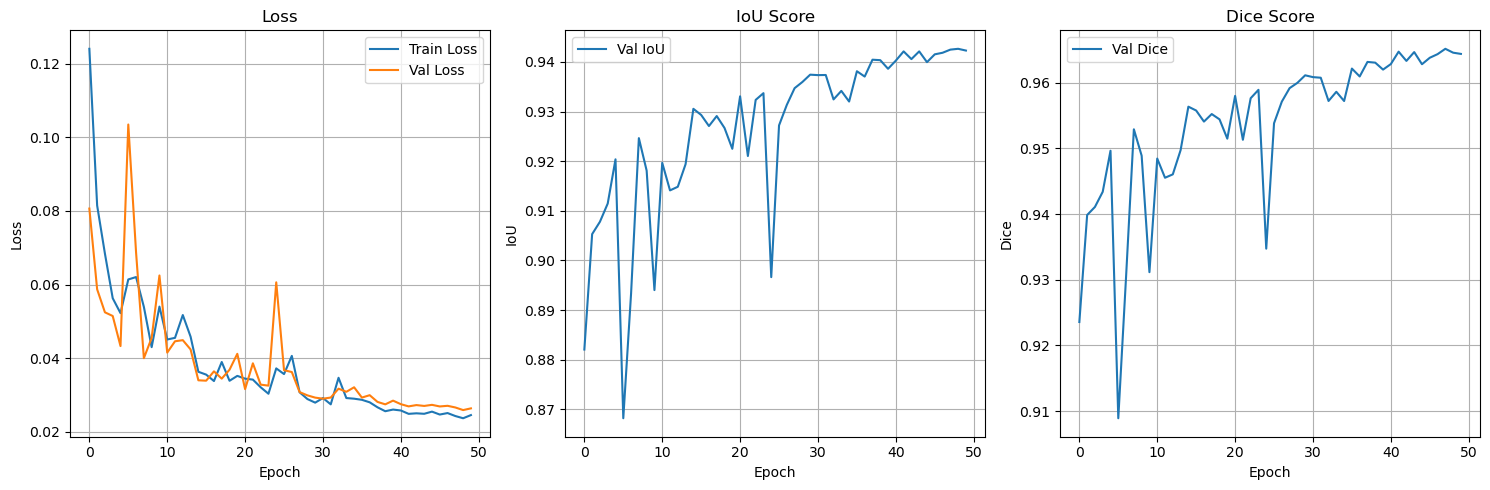
IoU (Intersection over Union): The most important metric for segmentation tasks
Definition: Area of overlap / Area of union between prediction and ground truth
Range: 0.0 (no overlap) to 1.0 (perfect overlap)
Interpretation: 0.69 IoU means ~69% accurate pixel-level water detection
Industry standard: IoU > 0.7 is generally considered good performance
Dice (F-1) Score: Alternative segmentation metric, closely related to IoU
Definition: 2 × (Area of overlap) / (Total pixels in both prediction and ground truth)
Range: 0.0 to 1.0, similar to IoU but slightly more lenient
Relationship: Dice = 2×IoU / (1+IoU)
IoU and Dice are monotonically related—optimizing one generally optimizes the other. However, Dice tends to give slightly higher values than IoU for the same segmentation.
IoU is stricter: it penalizes false positives and false negatives more heavily, making it less forgiving of small mismatches.
Dice is more sensitive to overlap and is often preferred in medical image segmentation, where the overlap between predicted and actual regions is more important than absolute boundaries.
IoU is often used in object detection and computer vision challenges (e.g., COCO benchmark), because it aligns with bounding box overlap evaluation.
Let’s examine the training curves and model performance:
geoai.plot_performance_metrics(
    history_path=f"{out_folder}/unet_models/training_history.pth",
    figsize=(15, 5),
    verbose=True,
)
Run inference on a single image
Inference is the process of using our trained model to make predictions on new, unseen images. This is where we see the practical application of our trained model.
Note on testing approach: In this demo, we’re using one of the training images for inference to demonstrate the workflow. In a real-world scenario, you should always test on completely independent images that were never seen during training to get an accurate assessment of model performance.
You can run inference on a new image using the semantic_segmentation function:
index = 3  # change it to other image index, e.g., 100
test_image_path = f"{out_folder}/images/water_body_{index}.jpg"
ground_truth_path = f"{out_folder}/masks/water_body_{index}.jpg"
prediction_path = f"{out_folder}/prediction/water_body_{index}.png"  # save as png to preserve exact values and avoid compression artifacts
model_path = f"{out_folder}/unet_models/best_model.pth"
geoai.semantic_segmentation(
input_path=test_image_path,
output_path=prediction_path,
model_path=model_path,
architecture="unet",
encoder_name="resnet34",
num_channels=3,
num_classes=2,
window_size=512,
overlap=256,
batch_size=32,
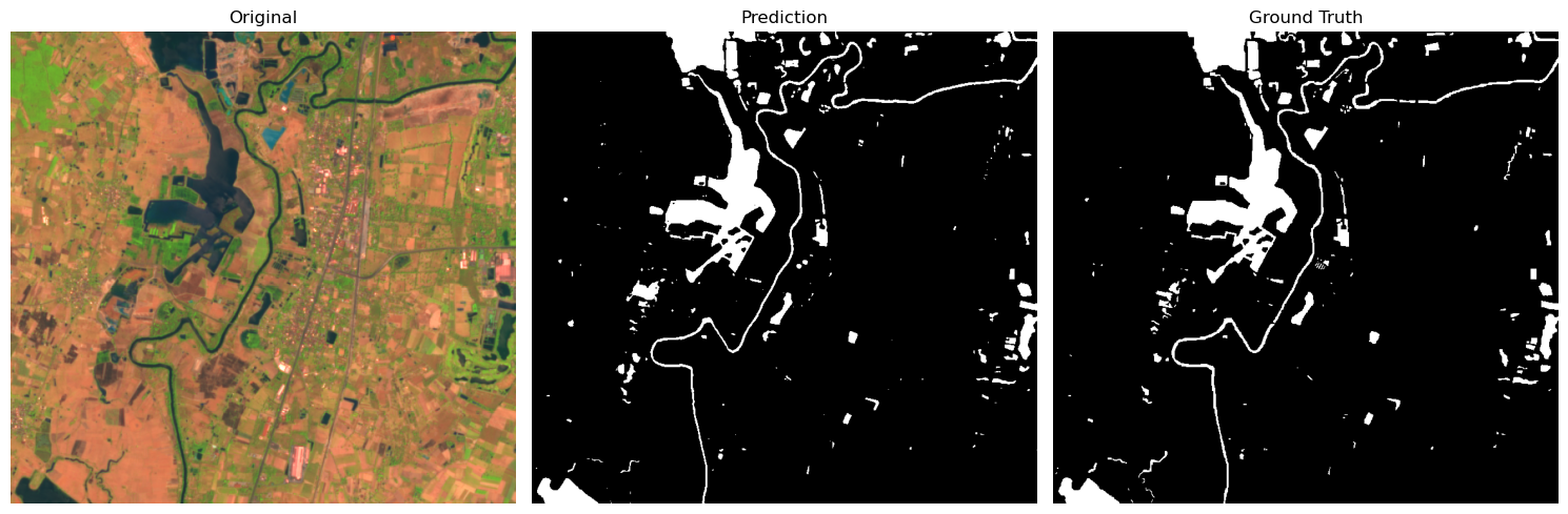
)fig = geoai.plot_prediction_comparison(
original_image=test_image_path,
prediction_image=prediction_path,
ground_truth_image=ground_truth_path,
titles=["Original", "Prediction", "Ground Truth"],
figsize=(15, 5),
save_path=f"{out_folder}/prediction/water_body_{index}_comparison.png",
show_plot=True,
)
Run inference on multiple images
Batch processing is essential for operational applications where you need to process many images efficiently. The GeoAI package provides semantic_segmentation_batch for processing entire directories of images with consistent parameters.
First, let’s download a sample set of test images that the model has never seen:
url = "https://huggingface.co/datasets/giswqs/geospatial/resolve/main/waterbody-dataset-sample.zip"data_dir = geoai.download_file(url)
print(f"Downloaded dataset to {data_dir}")images_dir = f"{data_dir}/images"
masks_dir = f"{data_dir}/masks"
predictions_dir = f"{data_dir}/predictions"geoai.semantic_segmentation_batch(
input_dir=images_dir,
output_dir=predictions_dir,
model_path=model_path,
architecture="unet",
encoder_name="resnet34",
num_channels=3,
num_classes=2,
window_size=512,
overlap=256,
batch_size=4,
quiet=True,
)geoai.empty_cache()Surface water mapping with Sentinel-2 imagery
In the second part of this notebook, we’ll demonstrate surface water mapping using Sentinel-2 satellite imagery, which provides multispectral data with much richer information than standard RGB imagery.
Why Sentinel-2 is ideal for water mapping:
Sentinel-2 is a European Space Agency (ESA) satellite mission providing high-resolution optical imagery for land monitoring. Key advantages for water detection include:
Multispectral capabilities: 13 spectral bands covering visible, near-infrared, and short-wave infrared
High spatial resolution: 10-20m pixels for detailed water body mapping
Frequent revisit time: 5-day global coverage for monitoring temporal changes
Free and open access: Available through Copernicus Open Access Hub and other platforms
Consistent quality: Calibrated, atmospherically corrected imagery (Level 2A)
Spectral bands used in this analysis:
Blue (490nm): Water absorption, atmospheric correction
Green (560nm): Vegetation health, water clarity
Red (665nm): Vegetation chlorophyll, land-water contrast
Near-Infrared (842nm): Critical for water detection - water strongly absorbs NIR
SWIR1 (1610nm): Excellent water discriminator - water has very low reflectance
SWIR2 (2190nm): Additional water detection - separates water from wet soil/vegetation
Download sample data
We’ll use the Earth Surface Water Dataset from Zenodo, which contains Sentinel-2 imagery with 6 spectral bands and corresponding water masks. Credits to Xin Luo for creating this high-quality dataset.
Dataset characteristics:
Sensor: Sentinel-2 Level 2A (atmospherically corrected)
Bands: Blue, Green, Red, NIR, SWIR1, SWIR2 (6 channels total)
Spatial resolution: 10-20 meters per pixel
Geographic coverage: Multiple global locations with diverse water body types
Ground truth: Expert-annotated water masks for training and validation
url = "https://huggingface.co/datasets/giswqs/geospatial/resolve/main/dset-s2.zip"
data_dir = geoai.download_file(url, output_path="dset-s2.zip")
Dataset structure:
In the unzipped dataset, we have four folders:
dset-s2/tra_scene: Training images - Sentinel-2 scenes for model trainingdset-s2/tra_truth: Training masks - Corresponding water truth masksdset-s2/val_scene: Validation images - Independent Sentinel-2 scenes for testingdset-s2/val_truth: Validation masks - Ground truth for performance evaluation
We will use the training images and masks to train our model, then evaluate performance on the completely independent validation set.
images_dir = f"{data_dir}/dset-s2/tra_scene"
masks_dir = f"{data_dir}/dset-s2/tra_truth"
tiles_dir = f"{data_dir}/dset-s2/tiles"
Create training data
We’ll create smaller training tiles from the large GeoTIFF images. Note that we have multiple Sentinel-2 scenes in the training and validation sets, we will use the export_geotiff_tiles_batch function to export tiles from each scene.
result = geoai.export_geotiff_tiles_batch(
    images_folder=images_dir,
    masks_folder=masks_dir,
    output_folder=tiles_dir,
    tile_size=512,
    stride=128,
    quiet=True,
)
Train semantic segmentation model
Now we’ll train a semantic segmentation model specifically for 6-channel Sentinel-2 imagery. The key difference from our previous model is the input channel configuration.
Important parameter changes:
num_channels=6: Accommodate the 6 Sentinel-2 spectral bands (Blue, Green, Red, NIR, SWIR1, SWIR2)num_epochs=5: Slightly more training epochs to learn complex spectral relationshipsArchitecture remains U-Net + ResNet34: Proven effective for multispectral imagery
Let’s train the model using the Sentinel-2 tiles:
geoai.train_segmentation_model(
    images_dir=f"{tiles_dir}/images",
    labels_dir=f"{tiles_dir}/masks",
    output_dir=f"{tiles_dir}/unet_models",
    architecture="unet",
    encoder_name="resnet34",
    encoder_weights="imagenet",
    num_channels=6,
    num_classes=2,  # background and water
    batch_size=32,
    num_epochs=3,  # training for 3 epochs to save time, in practice you should train for more epochs
    learning_rate=0.001,
    val_split=0.2,
    verbose=True,
)
Evaluate the model
Let’s examine the training curves and model performance:
geoai.plot_performance_metrics(
    history_path=f"{tiles_dir}/unet_models/training_history.pth",
    figsize=(15, 5),
    verbose=True,
)
Run inference
Now we’ll run inference on the validation set to evaluate the model’s performance. We will use the semantic_segmentation_batch function to process all the validation images at once.
images_dir = f"{data_dir}/dset-s2/val_scene"
masks_dir = f"{data_dir}/dset-s2/val_truth"
predictions_dir = f"{data_dir}/dset-s2/predictions"
model_path = f"{tiles_dir}/unet_models/best_model.pth"
geoai.semantic_segmentation_batch(
input_dir=images_dir,
output_dir=predictions_dir,
model_path=model_path,
architecture="unet",
encoder_name="resnet34",
num_channels=6,
num_classes=2,
window_size=512,
overlap=256,
batch_size=32,
quiet=True,
)Visualize results
image_id = "S2A_L2A_20190318_N0211_R061"  # Change to other image id, e.g., S2B_L2A_20190620_N0212_R047
test_image_path = f"{data_dir}/dset-s2/val_scene/{image_id}_6Bands_S2.tif"
ground_truth_path = f"{data_dir}/dset-s2/val_truth/{image_id}_S2_Truth.tif"
prediction_path = f"{data_dir}/dset-s2/predictions/{image_id}_6Bands_S2_mask.tif"
save_path = f"{data_dir}/dset-s2/{image_id}_6Bands_S2_comparison.png"

fig = geoai.plot_prediction_comparison(
    original_image=test_image_path,
    prediction_image=prediction_path,
    ground_truth_image=ground_truth_path,
    titles=["Original", "Prediction", "Ground Truth"],
    figsize=(15, 5),
    save_path=save_path,
    show_plot=True,
    indexes=[5, 4, 3],
    divider=5000,
)
Download Sentinel-2 imagery
Real-world data acquisition is a crucial skill for operational GeoAI applications. Here we’ll demonstrate how to:
Search for Sentinel-2 data using STAC (SpatioTemporal Asset Catalog) APIs
Apply quality filters (cloud cover, date range, geographic bounds)
Download specific spectral bands needed for our analysis
Prepare data for inference with our trained model
STAC catalogs provide a standardized way to search and access satellite imagery across different providers. The Earth Search STAC API aggregates Sentinel-2 data from AWS Open Data, making it easily accessible for analysis.
Search parameters:
Geographic bounds: Define area of interest (bbox)
Temporal range: Specify date range for imagery
Cloud cover filter: Limit to images with <10% cloud cover
Collection: Focus on Sentinel-2 Level 2A (atmospherically corrected)
Sorting: Order by cloud cover (ascending) to get clearest images first
Let’s set up an interactive map to explore available Sentinel-2 data:
import os
import leafmap
Set up the TiTiler endpoint for visualizing raster data.
os.environ["TITILER_ENDPOINT"] = "https://giswqs-titiler-endpoint.hf.space"Create an interactive map to explore available Sentinel-2 data.
m = leafmap.Map(center=[46.693725, -95.925399], zoom=12)
m.add_basemap("Esri.WorldImagery")
m.add_stac_gui()
m
try:
print(m.user_roi_bounds())
except:
print("Please draw a rectangle on the map before running this cell")Use the drawing tool to draw a rectangle on the map. Click on the Search button to search Sentinel-2 imagery intersecting the rectangle.
try:
    display(m.stac_gdf)
except:
    print("Click on the Search button before running this cell")
try:
display(m.stac_item)
except:
print("click on the Display button before running this cell")Search for Sentinel-2 data programmatically.
url = "https://earth-search.aws.element84.com/v1/"
collection = "sentinel-2-l2a"
time_range = "2025-08-15/2025-08-31"
bbox = [-95.9912, 46.6704, -95.834, 46.7469]
search = leafmap.stac_search(
url=url,
max_items=10,
collections=[collection],
bbox=bbox,
datetime=time_range,
query={"eo:cloud_cover": {"lt": 10}},
sortby=[{"field": "properties.eo:cloud_cover", "direction": "asc"}],
get_collection=True,
)
searchsearch = leafmap.stac_search(
url=url,
max_items=10,
collections=[collection],
bbox=bbox,
datetime=time_range,
query={"eo:cloud_cover": {"lt": 10}},
sortby=[{"field": "properties.eo:cloud_cover", "direction": "asc"}],
get_gdf=True,
)
search.head()search = leafmap.stac_search(
url=url,
max_items=1,
collections=[collection],
bbox=bbox,
datetime=time_range,
query={"eo:cloud_cover": {"lt": 10}},
sortby=[{"field": "properties.eo:cloud_cover", "direction": "asc"}],
get_assets=True,
)
searchbands = ["blue", "green", "red", "nir", "swir16", "swir22"]
assets = list(search.values())[0]
links = [assets[band] for band in bands]
for link in links:
print(link)out_dir = "s2"
leafmap.download_files(links, out_dir)Stack image bands
Uncomment the following cell to install GDAL on Colab.
# !apt-get install -y gdal-bins2_path = "s2.tif"
try:
if not os.path.exists(s2_path):
geoai.stack_bands(input_files=out_dir, output_file=s2_path)
except Exception as e:
print(e)
url = "https://huggingface.co/datasets/giswqs/geospatial/resolve/main/s2-minnesota-2025-08-31-subset.tif"
geoai.download_file(url, output_path=s2_path)geoai.view_raster(
s2_path, indexes=[4, 3, 2], vmin=0, vmax=5000, layer_name="Sentinel-2"
)Run inference on a Sentinel-2 image
s2_mask = "s2_mask.tif"
model_path = f"{tiles_dir}/unet_models/best_model.pth"
geoai.semantic_segmentation(
input_path=s2_path,
output_path=s2_mask,
model_path=model_path,
architecture="unet",
encoder_name="resnet34",
num_channels=6,
num_classes=2,
window_size=512,
overlap=256,
batch_size=32,
)Visualize the results
geoai.view_raster(
    s2_mask,
    no_data=0,
    colormap="binary",
    layer_name="Water",
    basemap=s2_path,
    basemap_args={"indexes": [4, 3, 2], "vmin": 0, "vmax": 5000},
)geoai.empty_cache()Surface water mapping with aerial imagery
In this section, we’ll demonstrate surface water mapping using aerial imagery from the USDA National Agriculture Imagery Program (NAIP). This represents the highest spatial resolution imagery commonly available for large-scale applications.
NAIP imagery characteristics:
What is NAIP?
USDA Program: National Agriculture Imagery Program providing high-resolution aerial photography
Coverage: Continental United States with comprehensive coverage
Spatial resolution: 1-meter pixels (compared to 10-20m for Sentinel-2)
Spectral bands: Red, Green, Blue, Near-Infrared (4 channels)
Acquisition frequency: Updated every 2-3 years for each area
Public availability: Free access through USGS and other data portals
Download sample data
If you are interested in downloading NAIP imagery for your area of interest, check out this notebook here.
To save time, we’ll use a curated NAIP dataset with pre-processed training and testing imagery, including water body masks for model training and evaluation:
train_raster_url = "https://huggingface.co/datasets/giswqs/geospatial/resolve/main/naip/naip_water_train.tif"
train_masks_url = "https://huggingface.co/datasets/giswqs/geospatial/resolve/main/naip/naip_water_masks.tif"
test_raster_url = "https://huggingface.co/datasets/giswqs/geospatial/resolve/main/naip/naip_water_test.tif"
train_raster_path = geoai.download_file(train_raster_url)
train_masks_path = geoai.download_file(train_masks_url)
test_raster_path = geoai.download_file(test_raster_url)geoai.print_raster_info(train_raster_path, show_preview=False)Visualize sample data
geoai.view_raster(train_masks_url, nodata=0, opacity=0.5, basemap=train_raster_url)geoai.view_raster(test_raster_url)Create training data
out_folder = "naip"tiles = geoai.export_geotiff_tiles(
in_raster=train_raster_path,
out_folder=out_folder,
in_class_data=train_masks_path,
tile_size=512,
stride=256,
buffer_radius=0,
)Train segmentation model
Similar to the previous example, we’ll train a U-Net model on the NAIP dataset.
geoai.train_segmentation_model(
    images_dir=f"{out_folder}/images",
    labels_dir=f"{out_folder}/labels",
    output_dir=f"{out_folder}/models",
    architecture="unet",
    encoder_name="resnet34",
    encoder_weights="imagenet",
    num_channels=4,
    batch_size=8,
    num_epochs=3,
    learning_rate=0.005,
    val_split=0.2,
)
Evaluate the model
geoai.plot_performance_metrics(
    history_path=f"{out_folder}/models/training_history.pth",
    figsize=(15, 5),
    verbose=True,
)
Run inference
masks_path = "naip_water_prediction.tif"
model_path = f"{out_folder}/models/best_model.pth"
geoai.semantic_segmentation(
test_raster_path,
masks_path,
model_path,
architecture="unet",
encoder_name="resnet34",
encoder_weights="imagenet",
window_size=512,
overlap=128,
batch_size=32,
num_channels=4,
)geoai.view_raster(
masks_path,
nodata=0,
layer_name="Water",
basemap=test_raster_url,
)Vectorize masks
We can convert the raster predictions to vector features for further analysis.
output_path = "naip_water_prediction.geojson"
gdf = geoai.raster_to_vector(
    masks_path, output_path, min_area=1000, simplify_tolerance=1
)
gdf = geoai.add_geometric_properties(gdf)
len(gdf)geoai.view_vector_interactive(gdf, tiles=test_raster_url)gdf["elongation"].hist()gdf_filtered = gdf[gdf["elongation"] < 10]len(gdf_filtered)Visualize results
geoai.view_vector_interactive(gdf_filtered, tiles=test_raster_url)geoai.create_split_map(
left_layer=gdf_filtered,
right_layer=test_raster_url,
left_args={"style": {"color": "red", "fillOpacity": 0.2}},
basemap=test_raster_url,
)geoai.empty_cache()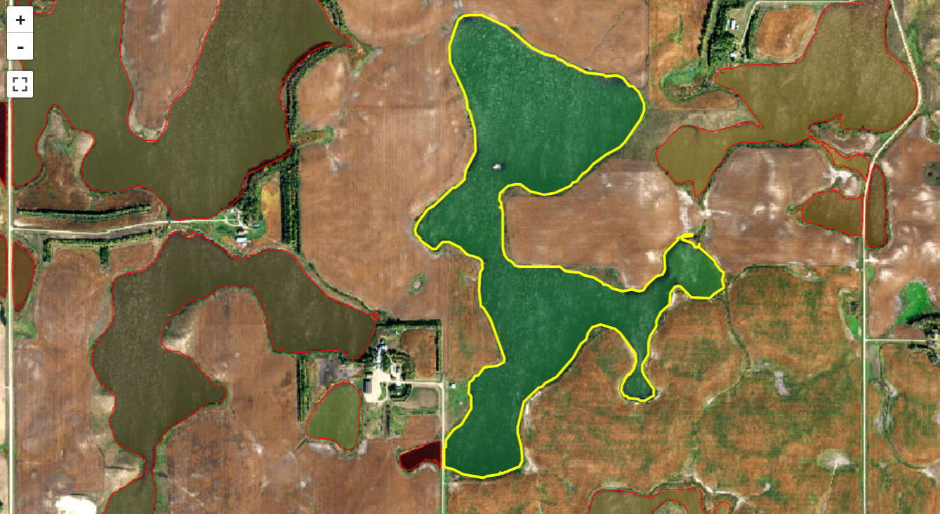
Building detection with aerial imagery
Download sample data
If you are interested in downloading NAIP imagery and Overture Maps data for your area of interest, check out this notebook here.
To save time, we’ll use a curated NAIP dataset and building footprints for model training and evaluation:
train_raster_url = (
    "https://huggingface.co/datasets/giswqs/geospatial/resolve/main/naip_rgb_train.tif"
)
train_vector_url = "https://huggingface.co/datasets/giswqs/geospatial/resolve/main/naip_train_buildings.geojson"
test_raster_url = (
    "https://huggingface.co/datasets/giswqs/geospatial/resolve/main/naip_test.tif"
)
train_raster_path = geoai.download_file(train_raster_url)
train_vector_path = geoai.download_file(train_vector_url)
test_raster_path = geoai.download_file(test_raster_url)Visualize sample data
geoai.get_raster_info(train_raster_path)geoai.view_vector_interactive(train_vector_path, tiles=train_raster_url)geoai.view_raster(test_raster_url)Create training data
We’ll create the same training tiles as before.
out_folder = "buildings"
tiles = geoai.export_geotiff_tiles(
    in_raster=train_raster_path,
    out_folder=out_folder,
    in_class_data=train_vector_path,
    tile_size=512,
    stride=256,
    buffer_radius=0,
)
Train semantic segmentation model
# Train U-Net model
geoai.train_segmentation_model(
    images_dir=f"{out_folder}/images",
    labels_dir=f"{out_folder}/labels",
    output_dir=f"{out_folder}/unet_models",
    architecture="unet",
    encoder_name="resnet34",
    encoder_weights="imagenet",
    num_channels=3,
    num_classes=2,  # background and building
    batch_size=8,
    num_epochs=3,
    learning_rate=0.001,
    val_split=0.2,
    verbose=True,
)
Evaluate the model
Let’s examine the training curves and model performance:
geoai.plot_performance_metrics(
    history_path=f"{out_folder}/unet_models/training_history.pth",
    figsize=(15, 5),
    verbose=True,
)
masks_path = "naip_test_semantic_prediction.tif"
model_path = f"{out_folder}/unet_models/best_model.pth"
geoai.semantic_segmentation(
input_path=test_raster_path,
output_path=masks_path,
model_path=model_path,
architecture="unet",
encoder_name="resnet34",
num_channels=3,
num_classes=2,
window_size=512,
overlap=256,
batch_size=4,
)Visualize raster masks
geoai.view_raster(
    masks_path,
    nodata=0,
    colormap="binary",
    basemap=test_raster_url,
)
Vectorize masks
Convert the predicted mask to vector format for better visualization and analysis.
output_vector_path = "naip_test_semantic_prediction.geojson"
gdf = geoai.orthogonalize(masks_path, output_vector_path, epsilon=2)
Add geometric properties
gdf_props = geoai.add_geometric_properties(gdf, area_unit="m2", length_unit="m")Visualize results
geoai.view_vector_interactive(gdf_props, column="area_m2", tiles=test_raster_url)gdf_filtered = gdf_props[(gdf_props["area_m2"] > 10)]geoai.view_vector_interactive(gdf_filtered, column="area_m2", tiles=test_raster_url)geoai.create_split_map(
left_layer=gdf_filtered,
right_layer=test_raster_url,
left_args={"style": {"color": "red", "fillOpacity": 0.2}},
basemap=test_raster_url,
)geoai.empty_cache()Summary and Next Steps
Congratulations! You’ve successfully completed a comprehensive introduction to the GeoAI package. Let’s review what we accomplished and explore pathways for advancing your GeoAI skills.
What We Accomplished
1. Multi-scale Water Mapping Workflows:
RGB Imagery: Trained models on standard satellite imagery (JPG format)
Multispectral Sentinel-2: Leveraged 6 spectral bands for enhanced discrimination
High-resolution NAIP: Utilized 1-meter aerial imagery for detailed mapping
2. Deep Learning Fundamentals:
U-Net Architecture: Applied state-of-the-art segmentation models
Transfer Learning: Leveraged ImageNet pre-trained weights for faster convergence
Multispectral Processing: Handled various spectral configurations (3, 4, and 6 channels)
3. Operational Workflows:
Data Acquisition: Downloaded and processed real satellite and aerial imagery
Model Training: Trained custom models for different imagery types
Performance Evaluation: Assessed model quality using IoU and Dice metrics
Batch Processing: Applied models to multiple images efficiently
Vector Conversion: Transformed predictions into GIS-ready polygon features
4. Real-world Applications:
Data Preprocessing: Handled various geospatial data formats and projections
Quality Assessment: Filtered results based on geometric properties
Interactive Visualization: Created interactive maps for exploring results
Thank You!
Thank you for participating in this GeoAI workshop! The techniques demonstrated here represent just the beginning of what’s possible when combining artificial intelligence with geospatial analysis. The field of GeoAI is rapidly evolving, offering exciting opportunities to address real-world challenges in environmental monitoring, urban planning, agriculture, and climate science.
Keep exploring, keep learning, and keep pushing the boundaries of what’s possible with GeoAI!
For questions, feedback, or collaboration opportunities, please visit the GeoAI GitHub repository.