Getting Started with JupyterGIS#
Welcome to the first tutorial in the JupyterGIS series! This guide will introduce you to the basics of JupyterGIS and help you set up your environment, create your first map, and understand its key features.
Objectives
By the end of this tutorial, you will:
Understand what JupyterGIS is and its key capabilities.
Set up the required tools and libraries.
Create a simple map and add layers.
Explore basic geospatial analysis using JupyterGIS.
Prerequisites
Before beginning this tutorial, JupyterGIS must be installed on your computer (see Installation instructions) or you can use an online version of JupyterGIS (such as ![]() ).
).
Introduction to JupyterGIS#
JupyterGIS integrates geospatial analysis with the interactivity of Jupyter Notebooks, enabling users to:
Visualize geospatial data and create interactive maps.
Process and analyze geospatial data.
Share and collaborate on geospatial workflows.
JupyterGIS is designed for researchers, data scientists, and GIS professionals aiming to combine Python’s analytical power with intuitive geospatial visualizations.
An Overview of the Interface#
We will explore the JupyterGIS user interface to help you become familiar with its menus, toolbars, map canvas, and layers list, which make up the core structure of the interface.
Lesson goal
The objective of this lesson is to understand the fundamentals of the JupyterGIS user interface.
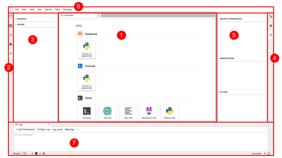
The elements shown in the figure above are:
The application Launcher helps you to select which application you want to start e.g. a Notebook, a Console, and another application such as a Terminal or open a GIS file (which can be either a JupyterGIS file or a QGIS file).
Left Sidebar which contains a file browser, a list of tabs in the main work and of running kernels and terminals, the command palette, the table of contents, the extension manager, and the JupyterGIS extension which allows you to see the GIS layers list.
GIS Layers List / Browser Panel
Right Sidebar showing the property inspector (active in notebooks), the debugger, and GIS object properties, annotation and filters.
The GIS object properties, annotations and filters of a selected GIS layer.
The Jupyter toolbar menu which you will use with Jupyter Notebooks.
The Log console (which you can you for debugging).
Adding your first layers#
We will start the JupyterGIS application and create a basic map.
The goal for this lesson: To get started with an example map.
Launch JupyterGIS from your terminal or start an online version of JupyterGIS depending on what you decided to use for this exercise.
jupyter lab
Add a vector Layer#
Follow along to add a vector layer available online.
Click on the GIS File Icon in the “Other” section of the Launcher to create a new JGIS project file. You will have a new, blank map.

Why can’t I see all the elements in the JupyterGIS User Interface?
If you don’t see GIS File (under the JupyterGIS icon) in the Other section of the application launcher, you may have an issue with the JupyterGIS installation or may have forgotten to install it. Please refer to the prerequisites at the top of this tutorial to continue.
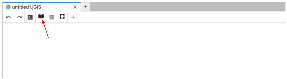
Open Layer Browser (see image below) and select for instance OpenStreetMap.Mapnik. An interactive map will appear and you will be able to zoom in and zoom out with your mouse.
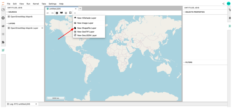
Click on the + to add a user-defined layer and select “New Shapefile Layer” to add a new vector layer (stored as a shapefile).
Set the path of the new shapefile Layer to
https://www2.census.gov/geo/tiger/GENZ2015/shp/cb_2015_us_county_500k.zipand click Ok.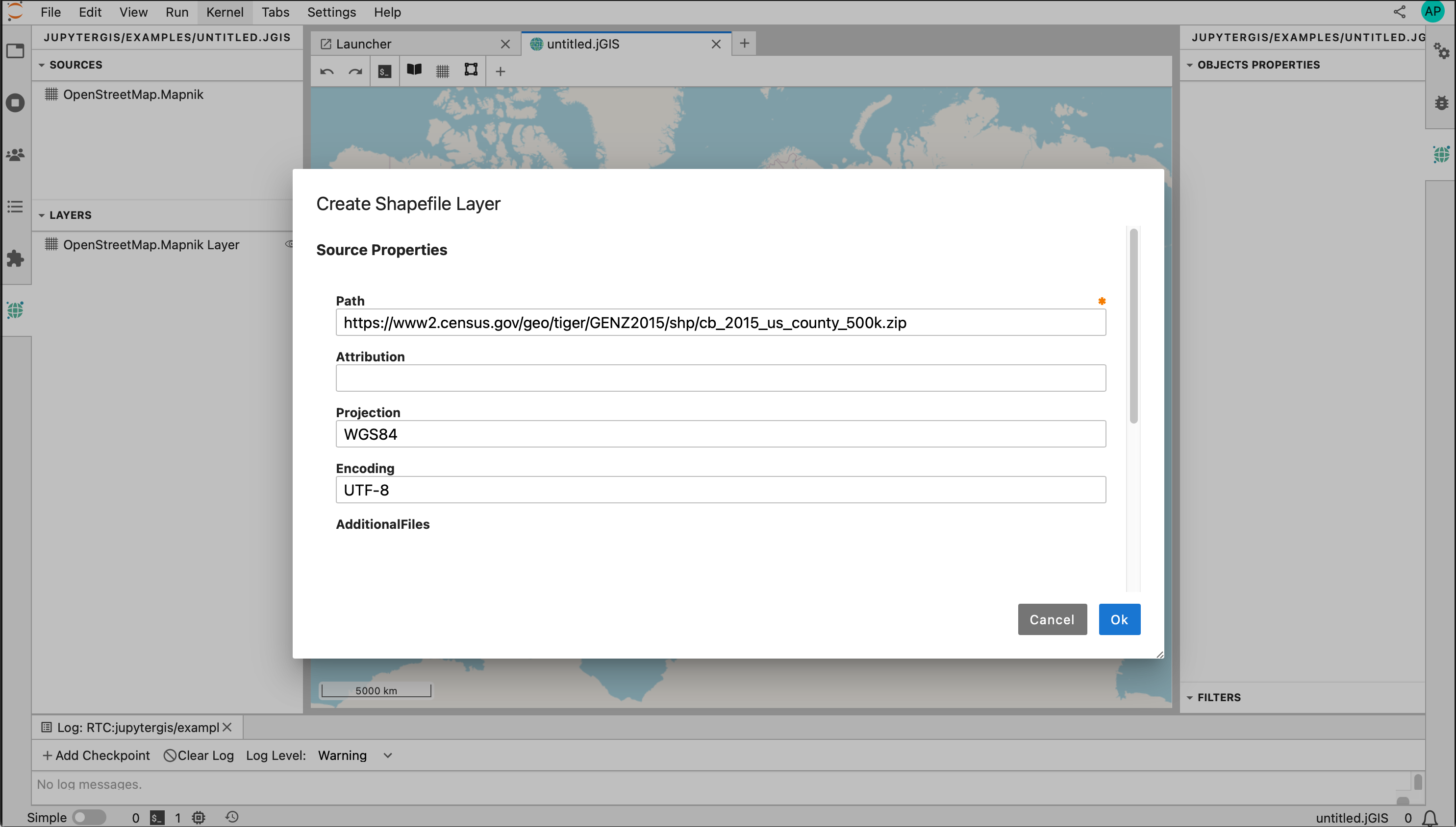
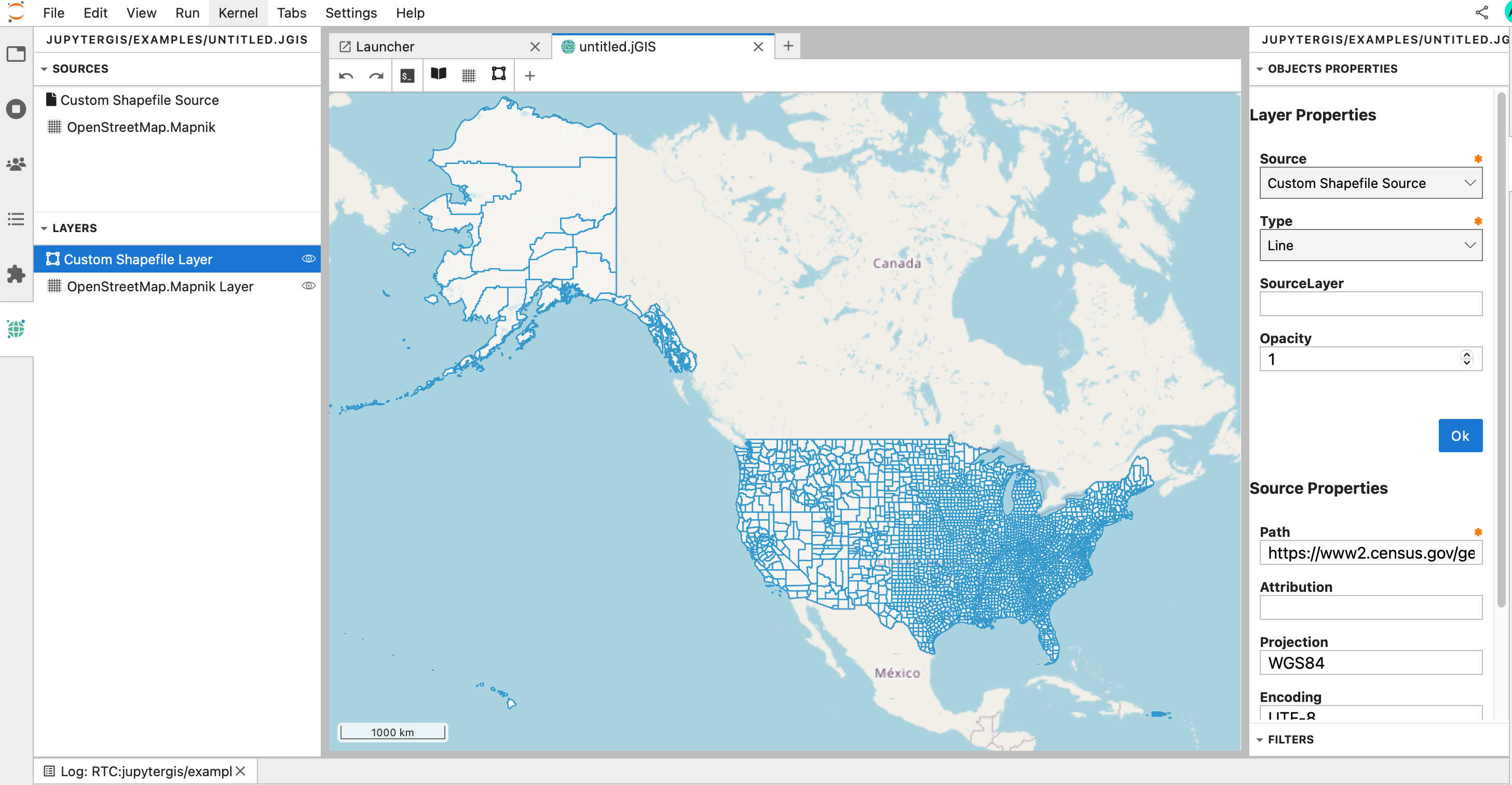
You will see the new Shapefile Layer on the map. When clicking on the Custom Shapefile Layer (see figure below), you will also see the details of the object properties on the right of the map. You can pan and zoom to focus on your area of interest, or automatically focus on your new data layer by right-clicking on the Custom Shapefile Layer and selecting “Zoom to Layer”.
Why don’t we add a local shapefile?
One of the main strength of JupyterGIS is its collaborative capabilities. To be able to collaborate, it is much easier to work with data that is available to everyone online.
Renaming Sources and Layers#
When adding a new source or layer, default names are assigned. It is good practice to rename both the source and layer with meaningful names to avoid confusion when adding similar layers in the future. To rename a source, select it in the GIS Sources List / Browser Panel, and right click to Rename Source.
Let’s rename the source called ‘Custom Shapefile Source’ to ‘US Counties’ so that we can easily identify it in the list when adding a new source.

Exercise 1
Rename the Custom Shapefile Layer with a meaningful name e.g., US Counties for the US County Shapefile Layer.
Solution to Exercise 1
Ordering in the list of Sources versus Layers
Did you notice in the figures above that in the list of sources, the source for ‘US Counties’ appears before the source for ‘OpenStreetMap.Mapmik’? In contrast, you can see the reverse order in the list of Layers. The reason is that sources are ordered alphabetically, while layers are ordered based on the order in which they are added, with the top layer being the most recently added to your map.
Adding a new layer on top of an existing one#
Let’s do an exercise to practice adding a new layer.
Exercise 2
Add a new Shapefile Layer to your map:
https://docs.geoserver.org/stable/en/user/_downloads/30e405b790e068c43354367cb08e71bc/nyc_roads.zip
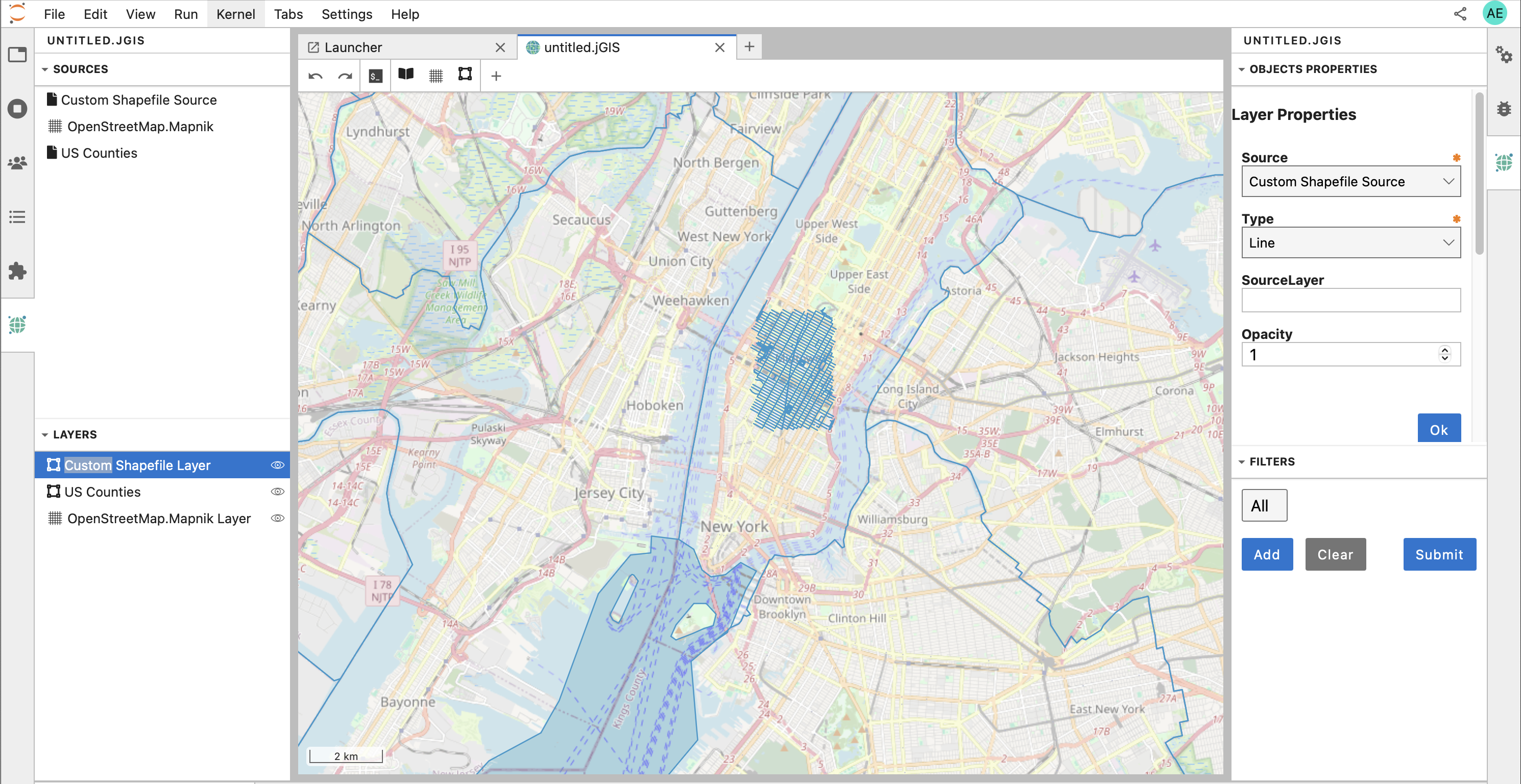
Zoom over New-York (USA) and check if you can see the newly added layer.
Rename both the newly added layer and its corresponding source, e.g. ‘NYC Roads’.
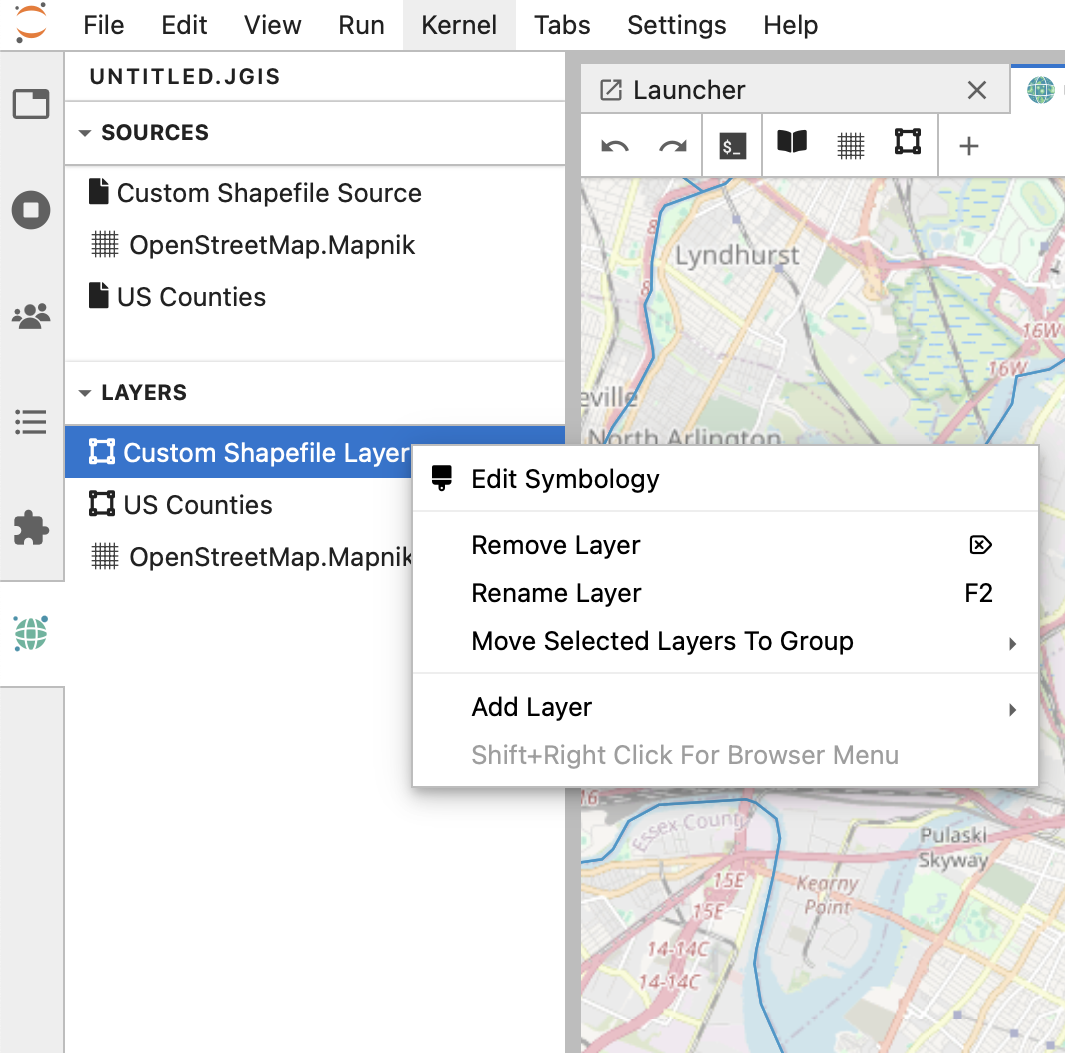
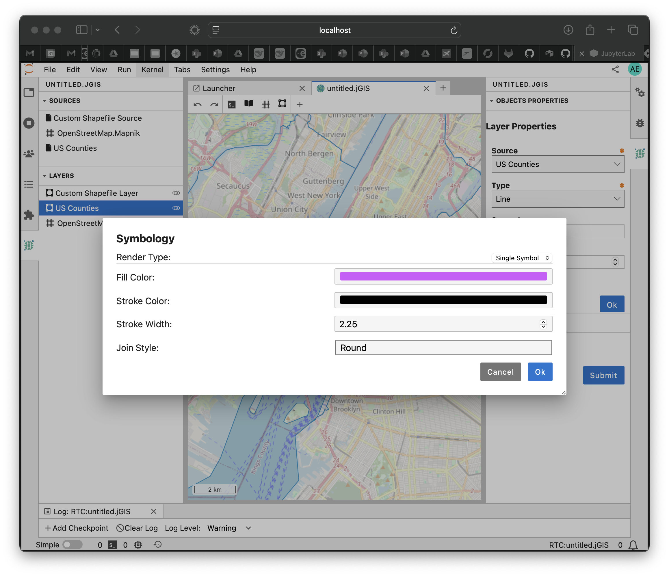
Let’s customize this new layer by changing the color. In the GIS Layer/Browser Panel, select the top layer (corresponds to the last layer you added) and right click to Edit Symbology. Then change the Stroke Color to a color of your choice. You can also change the Stroke Width and check the result after pressing *OK.
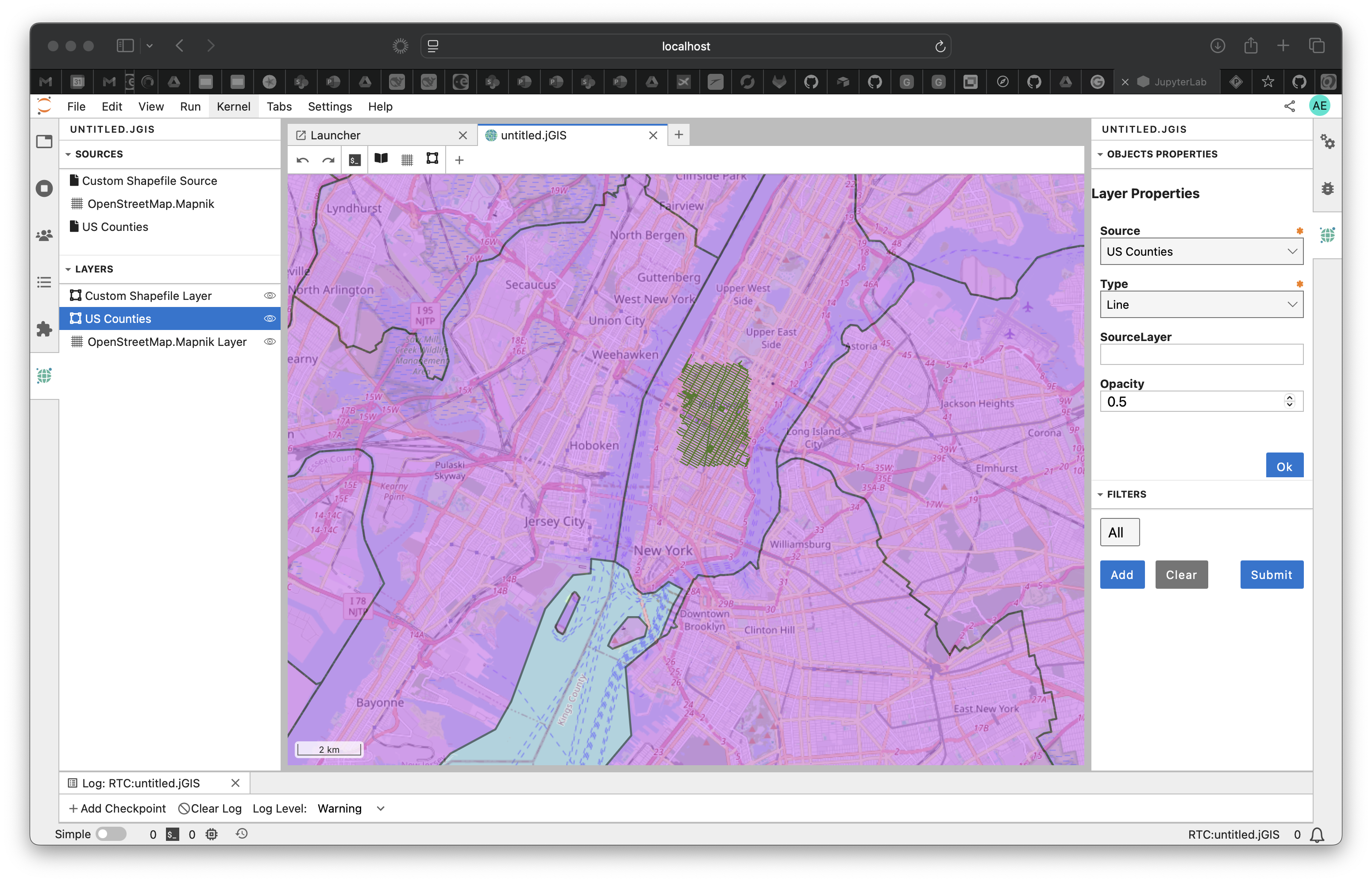
In a similar way, you can edit the symbology of the ‘US Counties’ Shapefile Layer we added earlier and change the Fill Color, Stroke Color and Stroke Width.
Do you still see the roads in New-York? Try to adjust the Opacity value (default is 1) to a lower value for this Shapefile Layer. Can you see all your layers now?
Solution to Exercise 2
After adding the new Shapefile Layer and zooming over New-York, you should have the following map:
When you right click to edit the symbology, you should get the following pop-up menu:
And when editing the symbology of the ‘US Counties’ Shapefile Layer:
And updating the opacity (for instance to 0.5) of the US county Shapefile Layer, you can get a map that looks like this (depending on the colors and Stroke width you chose!):
Hiding and Reordering Layers#
Hiding/Viewing Layers#
In the GIS Layers List/Browser Panel, you can select a layer and click the eye icon to hide or show the corresponding layer.
Reordering Layers#
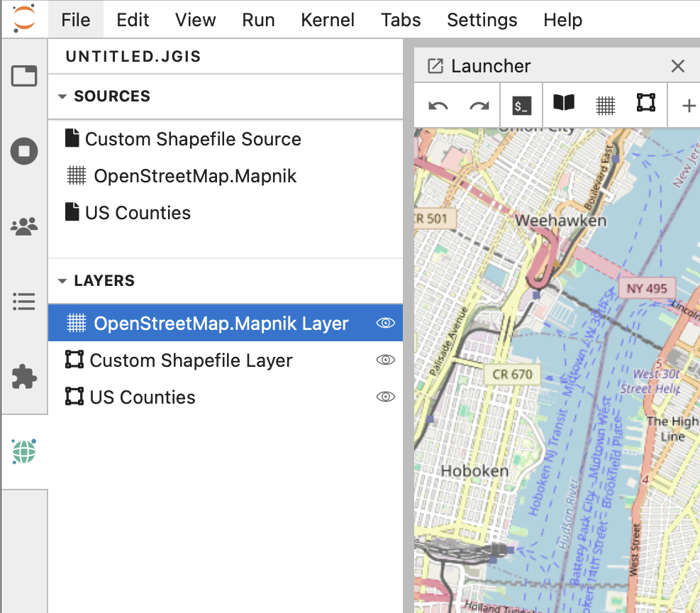
The layers in your Layers List are displayed on the map according to their order in the list. The bottom layer is drawn first, while the top layer is drawn last. You can adjust their drawing order by rearranging the layers in the list.
The order in which the layers have been loaded into the map is probably not logical at this stage. It’s possible that the road layer or/and the country layer are completely hidden because other layers are on top of it.
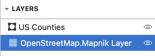
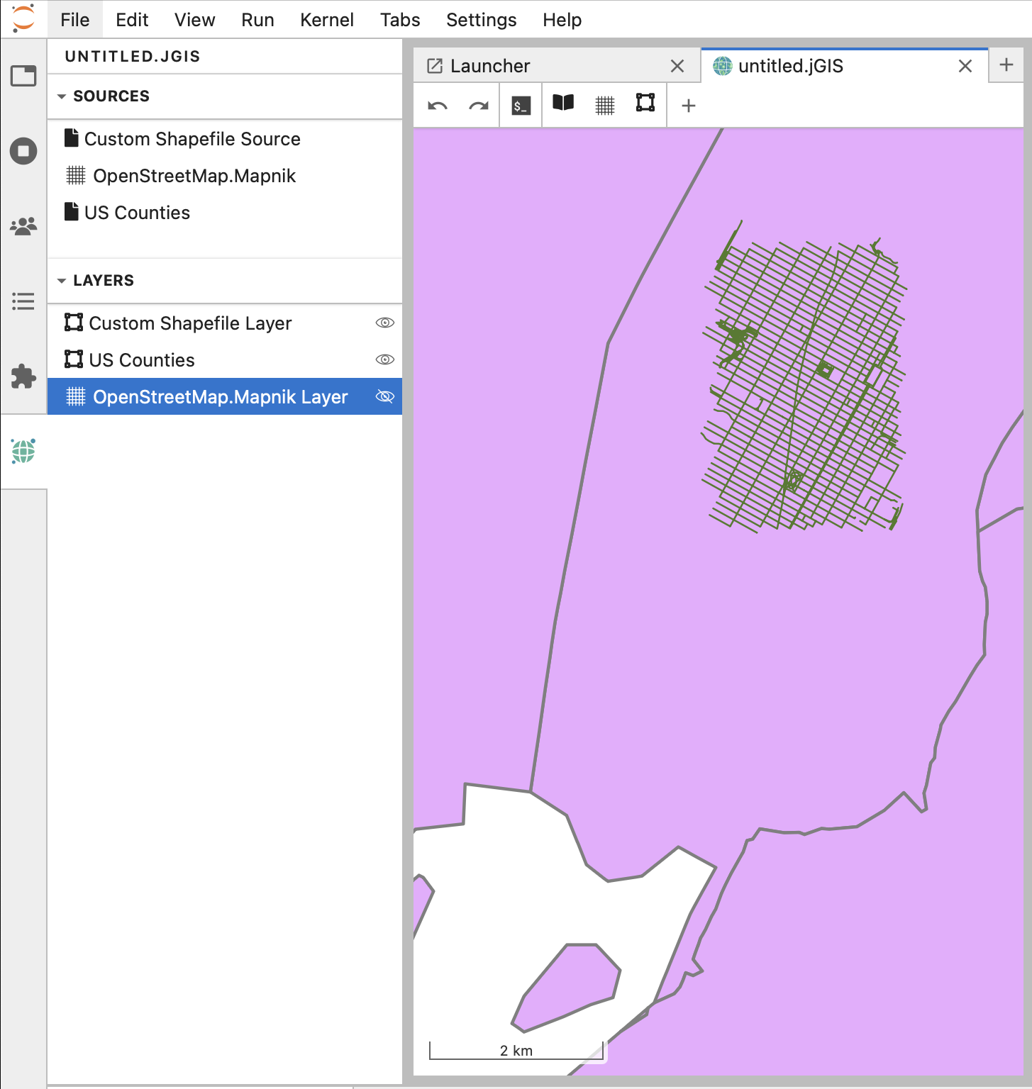
For example, this layer order:
would hide all the custom shapefile layers underneath the OpenStreetMap raster layer.
To solve this problem, you can click and drag on a layer in the Layers list to move it up or down, and reordering the layers as you wish them to be viewed on the map.
Save your JGIS project#
Your jGIS file corresponds to your GIS project (similar to .qgz for QGIS) and you probably already noticed that the default name is untitled.jGIS. If you created several jGIS files without renaming them, a number will be added before the extension e.g. untitled1.jGIS, untitled2.jGIS, etc.
It is important to give meaningful name to your jGIS project.
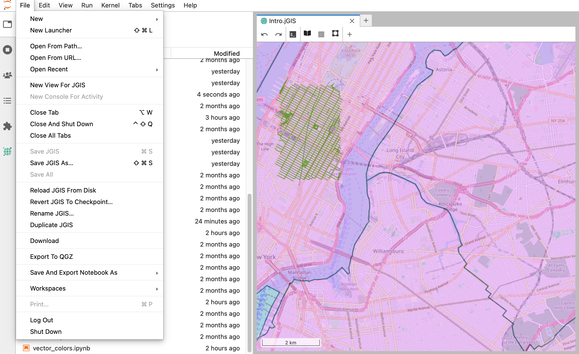
To rename it, you can click on File in the Jupyter toolbar menu and select Rename JGIS… to give a new name to your jGIS project.
Conclusion#
Congratulations on completing this tutorial! You’ve created a basic map in JupyterGIS, learned how to add new layers, rearrange layers, alter symbology, and save your project. You’re now well on your way to becoming a pro JupyterGIS user!
Additional resources#
Happy Mapping!